Module 2: Hands-on with pharmacogenomics data

Lab 2 Overview

Instructor(s) name(s) and contact information

Jermiah J. Joseph jermiah.joseph@uhn.ca
Almas Khan almas.khan@uhn.ca
Julia Nguyen julia.nguyen@uhn.ca

Learning goals

Understand the data structure of a PharmacoSet
Learn how to access features and metadata from a PharmacoSet
Learn how to plot batch effects using PCA and run correction method (SVA)
Learn how to filter out outliers and missing values

Learning objectives

Describe the use cases for PharmacoGx in Pharmacogenomics
Understand the structure of the CoreSet and PharmacoSet classes to facilitate their use in subsequent analyses
Download/load a PharmacoSet using PharmacoGx or orcestra.ca
Subset and filter a PharmacoSet by samples and/or treatments
Access the molecular features, dose-response and metadata contained within the PharmacoSet
Perform quality control on a PharmacoSet by identifying and removing outliers and missing values
Perform batch correction on a PharmacoSet using the sva package

Setup

Use Cases for PharmacoGx

Downloading Data from orcestra.ca

available <- PharmacoGx::availablePSets() |>
  data.table::as.data.table()

print(names(available))

## [1] "Dataset Name" "Date Created" "PSet Name"    "version"      "type"        
## [6] "publication"  "DOI"          "Download"

print(available[, c("Dataset Name", "PSet Name", "version")])

##     Dataset Name         PSet Name      version
##           <char>            <char>       <char>
##  1:         GDSC GDSC_2020(v2-8.2) 2020(v2-8.2)
##  2:         FIMM         FIMM_2016         2016
##  3:        Tavor        Tavor_2020         2020
##  4:        NCI60        NCI60_2021         2021
##  5:    UHNBreast    UHNBreast_2019         2019
##  6:         GDSC GDSC_2020(v1-8.2) 2020(v1-8.2)
##  7:        PRISM        PRISM_2020         2020
##  8:      BeatAML      BeatAML_2018         2018
##  9:         gCSI         gCSI_2019         2019
## 10:       CTRPv2       CTRPv2_2015         2015
## 11:         GRAY         GRAY_2017         2017
## 12:         CCLE         CCLE_2015         2015
## 13:         PDTX         PDTX_2019         2019
## 14:          GBM          GBM_scr2         2021
## 15:          GBM          GBM_scr3         2021
## 16:   NCISarcoma   NCISarcoma_2015         2015

. . .

The following function from PharmacoGx can be used to download any of the available PSets from orcestra.ca.

The command to do so is:

PharmacoGx::downloadPSet(
  name = "CCLE_2015",
  saveDir = "../psets", # change this directory as you see fit
  timeout = 3600,
  verbose = TRUE
)

# Note: this may take a while to download as the files are stored in
# Zenodo and are quite large

. . .

For convenience and in the interest of time, we have created a PharmacoSet to be used in this tutorial. We will be interacting with this dataset for the remainder of the tutorial.

pset <- CBWWorkshop2024::dummy_pset
pset

## <PharmacoSet>
## Name: dummy_pset 
## Date Created: Tue Oct 15 23:31:41 2024 
## Number of samples:  50 
## Molecular profiles: <MultiAssayExperiment> 
##    ExperimentList class object of length 2: 
##     [1] rnaseq.tpm : SummarizedExperiment with 100 rows and 50 columns 
##     [2] rnaseq.tpm.batch : SummarizedExperiment with 100 rows and 50 columns 
## Treatment response: <TreatmentResponseExperiment> 
##    dim:  4847 52 
##    assays(1): sensitivity 
##    rownames(4847): 1e-07:Ixabepilone:1 1e-06:Ixabepilone:1 ... 1000:Nelarabine:1 4000:Ifosfamide:1 
##    rowData(4): treatmentdose treatmentid tech_rep CONC1 
##    colnames(52): 786-O:1 A-498:1 A-549:1 ... UACC-257:1 UACC-62:1 UO-31:1 
##    colData(3): sampleid bio_rep PANEL 
##    metadata(0): none

Understanding the `PharmacoSet` Data Structure

The PharmacoSet class is a container for pharmacogenomic data.

This pharmacogenomic data is typically generated from high-throughput screening experiments where cell lines are treated with a panel of drugs at multiple doses and the response is measured using a molecular assay.

Pharmacogenomic data is located in a PharmacoSet within its slots, which are accessed using the @ operator.

slotNames(pset)

## [1] "treatmentResponse" "annotation"        "molecularProfiles"
## [4] "sample"            "treatment"         "datasetType"      
## [7] "perturbation"      "curation"

. . .

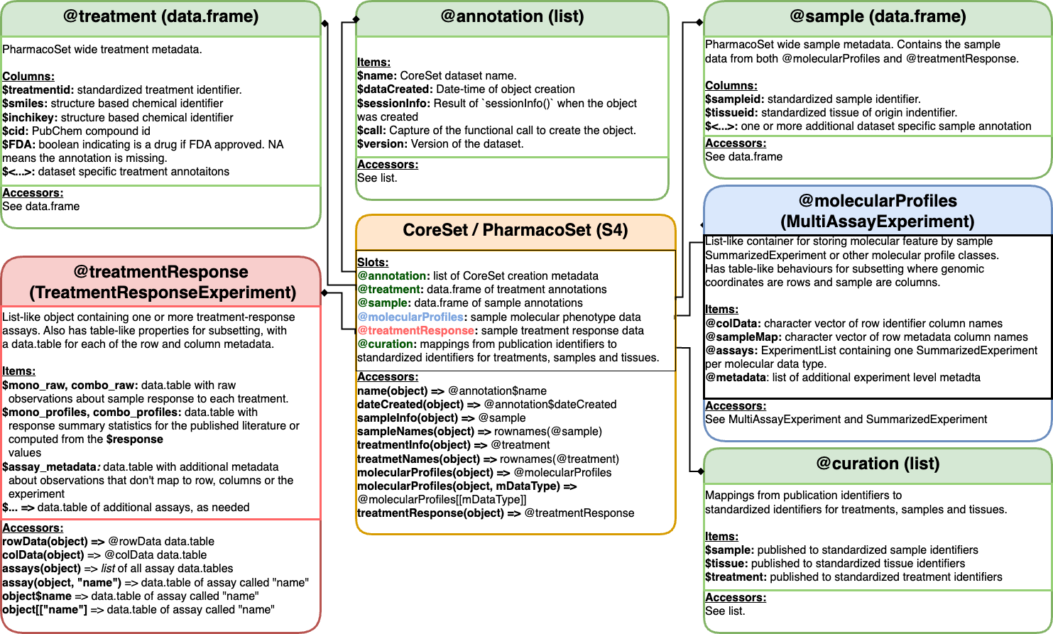
PharmacoSet class structure

Metadata

Metadata for cell-lines (samples) and drugs (treatments) are stored in the sample and treatment slots, respectively.

These are data frames with rows corresponding to samples or treatments and columns corresponding to metadata fields. The metadata fields are typically a combination of data from the original data source, and curated data from external sources such as Cellosaurus, DrugBank, and PubChem.

View the `sample` slot

We can access the sampleNames of the PharmacoSet:

PharmacoGx::sampleNames(pset)

##  [1] "NCI-H23"     "HOP-62"      "SNB-75"      "HL-60(TB)"   "A-549"      
##  [6] "SF268"       "SNB-19"      "SF295"       "OVCAR-5"     "U-251MG"    
## [11] "MCF-7"       "MDA-MB-231"  "MDA-MB-435"  "BT-549"      "SK-MEL-5"   
## [16] "MOLT-4"      "DU145"       "NCI-ADR-RES" "OVCAR-3"     "COLO 205"   
## [21] "SK-OV-3"     "CCRF-CEM"    "SR"          "IGROV-1"     "SW620"      
## [26] "Hs 578T"     "HCT 116"     "UACC-62"     "EKVX"        "HCT 15"     
## [31] "OVCAR-8"     "UACC-257"    "SF539"       "UO-31"       "M14"        
## [36] "KM12"        "T-47D"       "Malme-3M"    "Caki-1"      "A-498"      
## [41] "SK-MEL-28"   "RPMI-8226"   "NCI-H460"    "NCI-H322M"   "NCI-H226"   
## [46] "K-562"       "786-O"       "SK-MEL-2"    "HCC2998"     "NCI-H522"

. . .

To get all the metadata associated with the samples, we can access the sample slot:

pset@sample |> str()

## 'data.frame':    50 obs. of  7 variables:
##  $ sampleid            : chr  "NCI-H23" "HOP-62" "SNB-75" "HL-60(TB)" ...
##  $ tissueid            : chr  "Lung" "Lung" "CNS/Brain" "Myeloid" ...
##  $ cellosaurus_disease : chr  "Lung adenocarcinoma" "Lung adenocarcinoma" "Glioblastoma" "Acute myeloid leukemia" ...
##  $ cellosaurus_id      : chr  "CVCL_1547" "CVCL_1285" "CVCL_1706" "CVCL_A794" ...
##  $ NCI_ALMANAC.sampleid: chr  "NCI-H23" "HOP-62" "SNB-75" "HL-60(TB)" ...
##  $ NCI_ALMANAC.disease : chr  "Non-Small Cell Lung Cancer" "Non-Small Cell Lung Cancer" "CNS Cancer" "Leukemia" ...
##  $ pharmacodb_cid      : chr  "NCIH23_1085_2019" "HOP62_561_2019" "SNB75_1430_2019" "HL-60(TB)6502021_" ...

We can see from the sample slot that there are 50 samples in this PharmacoSet.

View the `treatment` slot

Similar to the sample, we can access the treatmentNames of the PharmacoSet:

PharmacoGx::treatmentNames(pset) |> head()

## [1] "Ixabepilone" "Clofarabine" "Dasatinib"   "Vincristine" "Imiquimod"  
## [6] "Paclitaxel"

. . .

To get all the metadata associated with the treatments, we can access the treatment slot:

pset@treatment |> str()

## 'data.frame':    22 obs. of  3 variables:
##  $ treatmentid: chr  "Ixabepilone" "Clofarabine" "Dasatinib" "Vincristine" ...
##  $ cid        : int  6445540 119182 3062316 5978 57469 36314 13342 54611422 2141 176871 ...
##  $ inchikey   : chr  "FABUFPQFXZVHFB-PVYNADRNSA-N" "WDDPHFBMKLOVOX-UHFFFAOYSA-N" "ZBNZXTGUTAYRHI-UHFFFAOYSA-N" "" ...

There are also 22 treatments used.

Molecular Profiles

In PharmacoGx, molecular profiles refer to any data that is measured on the samples in the PharmacoSet. This can include gene expression, copy number, mutation, or any other type of data that can be measured on a sample.

Each Molecular Data Type (mDataType) is stored in a SummarizedExperiment. All the SummarizedExperiment objects are stored in a container called a MultiAssayExperiment which can be accessed through the molecularProfiles slot.

`MultiAssayExperiment` and `SummarizedExperiment`

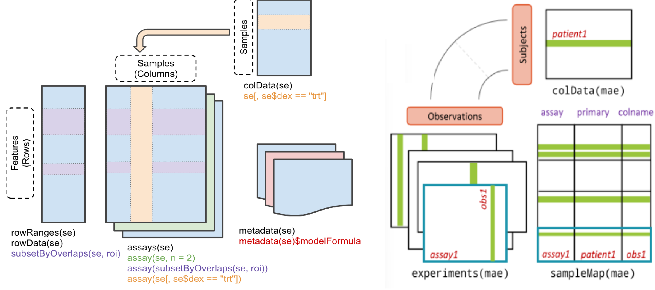
SummarizedExperiment and MultiAssayExperiment classes.

View the `molecularProfiles` slot

pset@molecularProfiles

## A MultiAssayExperiment object of 2 listed
##  experiments with user-defined names and respective classes.
##  Containing an ExperimentList class object of length 2:
##  [1] rnaseq.tpm: SummarizedExperiment with 100 rows and 50 columns
##  [2] rnaseq.tpm.batch: SummarizedExperiment with 100 rows and 50 columns
## Functionality:
##  experiments() - obtain the ExperimentList instance
##  colData() - the primary/phenotype DataFrame
##  sampleMap() - the sample coordination DataFrame
##  `$`, `[`, `[[` - extract colData columns, subset, or experiment
##  *Format() - convert into a long or wide DataFrame
##  assays() - convert ExperimentList to a SimpleList of matrices
##  exportClass() - save data to flat files

Treatment Response

The treatment response data was traditionally stored in a list. To accelerate analysis, we have developed a new class called the TreatmentResponseExperiment (TRE) which has been specifically designed to handle high dimensional biological stimulus-response data.

View the `treatmentResponse` slot

pset@treatmentResponse

## <TreatmentResponseExperiment> 
##    dim:  4847 52 
##    assays(1): sensitivity 
##    rownames(4847): 1e-07:Ixabepilone:1 1e-06:Ixabepilone:1 ... 1000:Nelarabine:1 4000:Ifosfamide:1 
##    rowData(4): treatmentdose treatmentid tech_rep CONC1 
##    colnames(52): 786-O:1 A-498:1 A-549:1 ... UACC-257:1 UACC-62:1 UO-31:1 
##    colData(3): sampleid bio_rep PANEL 
##    metadata(0): none

. . .

To view all the methods available for the TreatmentResponseExperiment class, we can use the methods function:

methods(class = "TreatmentResponseExperiment")

##  [1] [                   [[                  [[<-               
##  [4] $                   $<-                 aggregate          
##  [7] assay               assay<-             assayCols          
## [10] assayIndex          assayKeys           assayNames         
## [13] assays              assays<-            buildComboProfiles 
## [16] coerce              colData             colData<-          
## [19] colIDs              colMeta             colnames           
## [22] computeZIPdelta     dim                 dimnames           
## [25] endoaggregate       getIntern           idCols             
## [28] mergeAssays         metadata            metadata<-         
## [31] names               reindex             rowData            
## [34] rowData<-           rowIDs              rowMeta            
## [37] rownames            show                subset             
## [40] treatmentResponse<- updateObject       
## see '?methods' for accessing help and source code

Subsetting a `PharmacoSet`

Subset by `sampleNames` and/or `treatmentNames`

When subsetting a PharmacoSet object by sample names, both the MultiAssayExperiment and TreatmentResponseExperiment objects will be subsetted so all their internal Experiments only contain data for the samples of interest.

However, when subsetting by treatment names, only the TRE object will be subsetted.

. . .

PharmacoGx::subsetBySample(
  pset,
  sample = PharmacoGx::sampleNames(pset)[1:5]
)

## <PharmacoSet>
## Name: dummy_pset 
## Date Created: Tue Oct 15 23:31:41 2024 
## Number of samples:  5 
## Molecular profiles: <MultiAssayExperiment> 
##    ExperimentList class object of length 2: 
##     [1] rnaseq.tpm : SummarizedExperiment with 100 rows and 5 columns 
##     [2] rnaseq.tpm.batch : SummarizedExperiment with 100 rows and 5 columns 
## Treatment response: <TreatmentResponseExperiment> 
##    dim:  4440 4 
##    assays(1): sensitivity 
##    rownames(4440): 1e-07:Ixabepilone:1 1e-06:Ixabepilone:1 ... 1000:Nelarabine:1 4000:Ifosfamide:1 
##    rowData(4): treatmentdose treatmentid tech_rep CONC1 
##    colnames(4): A-549:1 HOP-62:1 NCI-H23:1 SNB-75:1 
##    colData(3): sampleid bio_rep PANEL 
##    metadata(0): none

PharmacoGx::subsetByTreatment(
  pset,
  treatment = PharmacoGx::treatmentNames(pset)[1:5]
)

## <PharmacoSet>
## Name: dummy_pset 
## Date Created: Tue Oct 15 23:31:41 2024 
## Number of samples:  50 
## Molecular profiles: <MultiAssayExperiment> 
##    ExperimentList class object of length 2: 
##     [1] rnaseq.tpm : SummarizedExperiment with 100 rows and 50 columns 
##     [2] rnaseq.tpm.batch : SummarizedExperiment with 100 rows and 50 columns 
## Treatment response: <TreatmentResponseExperiment> 
##    dim:  883 51 
##    assays(1): sensitivity 
##    rownames(883): 1e-07:Ixabepilone:1 1e-06:Ixabepilone:1 ... 7:Clofarabine:1 10:Clofarabine:1 
##    rowData(4): treatmentdose treatmentid tech_rep CONC1 
##    colnames(51): 786-O:1 A-498:1 A-549:1 ... UACC-257:1 UACC-62:1 UO-31:1 
##    colData(3): sampleid bio_rep PANEL 
##    metadata(0): none

Subsetting using `sample` and `treatment` metadata

The utility of the metadata slots in the PharmacoSet class

unique(pset@sample$tissueid)

##  [1] "Lung"                 "CNS/Brain"            "Myeloid"             
##  [4] "Ovary/Fallopian Tube" "Breast"               "Skin"                
##  [7] "Lymphoid"             "Prostate"             "Bowel"               
## [10] "Kidney"               "Pleura"

tissues_of_interest <- c("Kidney")

(samples_of_interest <- pset@sample[
  pset@sample$tissueid %in% tissues_of_interest,
  "sampleid"
]
)

## [1] "UO-31"  "Caki-1" "A-498"  "786-O"

PharmacoGx::subsetBySample(
  pset,
  samples_of_interest
)

## <PharmacoSet>
## Name: dummy_pset 
## Date Created: Tue Oct 15 23:31:41 2024 
## Number of samples:  4 
## Molecular profiles: <MultiAssayExperiment> 
##    ExperimentList class object of length 2: 
##     [1] rnaseq.tpm : SummarizedExperiment with 100 rows and 4 columns 
##     [2] rnaseq.tpm.batch : SummarizedExperiment with 100 rows and 4 columns 
## Treatment response: <TreatmentResponseExperiment> 
##    dim:  4285 4 
##    assays(1): sensitivity 
##    rownames(4285): 1e-07:Ixabepilone:1 1e-06:Ixabepilone:1 ... 1000:Nelarabine:1 4000:Ifosfamide:1 
##    rowData(4): treatmentdose treatmentid tech_rep CONC1 
##    colnames(4): 786-O:1 A-498:1 Caki-1:1 UO-31:1 
##    colData(3): sampleid bio_rep PANEL 
##    metadata(0): none

A concise way to subset by sample in one step:

PharmacoGx::subsetBySample(
  pset,
  sample = pset@sample[
    pset@sample$tissueid == "Kidney",
    "sampleid"
  ]
)

## <PharmacoSet>
## Name: dummy_pset 
## Date Created: Tue Oct 15 23:31:41 2024 
## Number of samples:  4 
## Molecular profiles: <MultiAssayExperiment> 
##    ExperimentList class object of length 2: 
##     [1] rnaseq.tpm : SummarizedExperiment with 100 rows and 4 columns 
##     [2] rnaseq.tpm.batch : SummarizedExperiment with 100 rows and 4 columns 
## Treatment response: <TreatmentResponseExperiment> 
##    dim:  4285 4 
##    assays(1): sensitivity 
##    rownames(4285): 1e-07:Ixabepilone:1 1e-06:Ixabepilone:1 ... 1000:Nelarabine:1 4000:Ifosfamide:1 
##    rowData(4): treatmentdose treatmentid tech_rep CONC1 
##    colnames(4): 786-O:1 A-498:1 Caki-1:1 UO-31:1 
##    colData(3): sampleid bio_rep PANEL 
##    metadata(0): none

Computing over a `TreatmentResponseExperiment`

The TreatmentResponseExperiment class has been designed to facilitate more than just storing data efficiently. Once the data is curated and stored safely inside our object, we are ready to start answering questions.

First, let’s extract the TRE to work with:

tre <- pset@treatmentResponse
show(tre)

## <TreatmentResponseExperiment> 
##    dim:  4847 52 
##    assays(1): sensitivity 
##    rownames(4847): 1e-07:Ixabepilone:1 1e-06:Ixabepilone:1 ... 1000:Nelarabine:1 4000:Ifosfamide:1 
##    rowData(4): treatmentdose treatmentid tech_rep CONC1 
##    colnames(52): 786-O:1 A-498:1 A-549:1 ... UACC-257:1 UACC-62:1 UO-31:1 
##    colData(3): sampleid bio_rep PANEL 
##    metadata(0): none

Aggregating over the `TreatmentResponseExperiment`

The aggregate function is a powerful tool that allows us to summarize the data in a TreatmentResponseExperiment object.

tre |>
  aggregate(
    assay = "sensitivity",
    N = .N,
    by = c("treatmentid", "treatmentdose", "sampleid", "bio_rep")
  )

##       treatmentid treatmentdose sampleid bio_rep     N
##            <char>         <num>   <char>   <int> <int>
##    1: Ixabepilone         1e-07    786-O       1     1
##    2: Ixabepilone         1e-07    A-498       1     1
##    3: Ixabepilone         1e-07    A-549       1     1
##    4: Ixabepilone         1e-07   BT-549       1     1
##    5: Ixabepilone         1e-07 COLO 205       1     1
##   ---                                                 
## 9036:  Ifosfamide         4e+03    T-47D       1     1
## 9037:  Ifosfamide         4e+03  U-251MG       1     1
## 9038:  Ifosfamide         4e+03 UACC-257       1     1
## 9039:  Ifosfamide         4e+03  UACC-62       1     1
## 9040:  Ifosfamide         4e+03    UO-31       1     1

You can also use the subset function to subset the TreatmentResponseExperiment object before performing aggregate.

Additionally, you can even subset over the result of an aggregate operation.

tre |>
  subset(treatmentid %in% c("Doxorubicin", "Ixabepilone")) |>
  aggregate(
    assay = "sensitivity",
    N = .N,
    by = c("treatmentid", "treatmentdose", "sampleid", "bio_rep")
  ) |>
  subset(N > 1 & sampleid == "A-498")

##     treatmentid treatmentdose sampleid bio_rep     N
##          <char>         <num>   <char>   <int> <int>
##  1: Ixabepilone         3e-05    A-498       1     2
##  2: Doxorubicin         5e-05    A-498       1   102
##  3: Ixabepilone         3e-04    A-498       1     2
##  4: Doxorubicin         5e-04    A-498       1   102
##  5: Ixabepilone         3e-03    A-498       1    10
##  6: Doxorubicin         5e-03    A-498       1   122
##  7: Ixabepilone         3e-02    A-498       1     8
##  8: Doxorubicin         5e-02    A-498       1   122
##  9: Ixabepilone         3e-01    A-498       1     8
## 10: Doxorubicin         5e-01    A-498       1   122
## 11: Doxorubicin         5e+00    A-498       1   102

Plotting the number of replicates

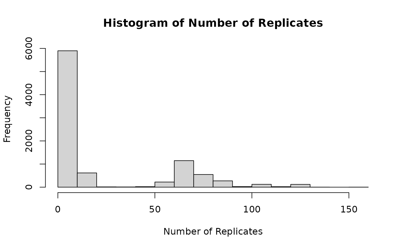
The last two examples have shown that there are technical replicates in the data. We can visualize the number of replicates using a histogram.

tre |>
  aggregate(
    assay = "sensitivity",
    N = .N,
    by = c("treatmentid", "treatmentdose", "sampleid", "bio_rep")
  ) |>
  with(
    expr = hist(
      N,
      main = "Histogram of Number of Replicates",
      xlab = "Number of Replicates"
    )
  )

Summarize over technical replicates

Depending on the experiment design, you will need to choose how you want to proceed with the data.

One common approach is to summarize the technical replicates into a single value, this can be done by taking the mean, median, or any other summary statistic.

`Endoaggregate`

In the interest of computation time and resources, we want to summarize the technical replicates into a single value and store that result inside the TreatmentResponseExperiment.

For this, we have developed the endoaggregate method.

This method will perform similar to the aggregate method, but will return a TreatmentResponseExperiment object with the summarized data as another assay.

new_tre <- tre |>
  endoaggregate(
    N = .N,
    assay = "sensitivity",
    target = "tech_rep_counts",
    by = c("treatmentid", "treatmentdose", "sampleid", "bio_rep")
  )
show(new_tre)

## <TreatmentResponseExperiment> 
##    dim:  4847 52 
##    assays(2): sensitivity tech_rep_counts 
##    rownames(4847): 1e-07:Ixabepilone:1 1e-06:Ixabepilone:1 ... 1000:Nelarabine:1 4000:Ifosfamide:1 
##    rowData(4): treatmentdose treatmentid tech_rep CONC1 
##    colnames(52): 786-O:1 A-498:1 A-549:1 ... UACC-257:1 UACC-62:1 UO-31:1 
##    colData(3): sampleid bio_rep PANEL 
##    metadata(0): none

head(new_tre$tech_rep_counts[order(-N)])

##    treatmentdose treatmentid    sampleid bio_rep     N
##            <num>      <char>      <char>   <int> <int>
## 1:         0.005 Doxorubicin     HCT 116       1   153
## 2:         0.050 Doxorubicin     HCT 116       1   153
## 3:         0.500 Doxorubicin     HCT 116       1   153
## 4:         0.005 Doxorubicin NCI-ADR-RES       1   132
## 5:         0.050 Doxorubicin NCI-ADR-RES       1   132
## 6:         0.500 Doxorubicin NCI-ADR-RES       1   132

Let’s use this method to summarize the technical replicates by taking the mean of the viability values for each unique combination of treatmentid, treatmentdose, sampleid, and bio_rep.

tre_avged <- tre |>
  endoaggregate(
    viability = mean(viability),
    assay = "sensitivity",
    target = "mean_sensitivity",
    by = c("treatmentid", "treatmentdose", "sampleid", "bio_rep")
  )
str(tre_avged$mean_sensitivity)

## Classes 'data.table' and 'data.frame':   9040 obs. of  5 variables:
##  $ treatmentdose: num  1e-07 1e-07 1e-07 1e-07 1e-07 1e-07 1e-07 1e-07 1e-07 1e-07 ...
##  $ treatmentid  : chr  "Ixabepilone" "Ixabepilone" "Ixabepilone" "Ixabepilone" ...
##  $ sampleid     : chr  "786-O" "A-498" "A-549" "BT-549" ...
##  $ bio_rep      : int  1 1 1 1 1 1 1 1 1 1 ...
##  $ viability    : num  98 99.7 99.3 96 103.7 ...
##  - attr(*, "sorted")= chr [1:4] "treatmentdose" "treatmentid" "sampleid" "bio_rep"
##  - attr(*, ".internal.selfref")=<externalptr>

Computing profiles

tre_profiled <- tre_avged |>
  endoaggregate(
    {
      fit <- PharmacoGx::logLogisticRegression(treatmentdose, viability)
      IC50 <- PharmacoGx::computeIC50(treatmentdose, Hill_fit = fit)
      AAC <- PharmacoGx::computeAUC(treatmentdose, Hill_fit = fit, area.type = "Fitted")
      list(
        HS = fit[["HS"]], E_inf = fit[["E_inf"]] / 100, EC50 = fit[["EC50"]],
        Rsq = as.numeric(unlist(attributes(fit))),
        AAC = AAC,
        IC50 = IC50
      )
    },
    assay = "mean_sensitivity",
    subset = treatmentid %in% rowData(tre_avged)[, unique(treatmentid)][1:3],
    by = c("treatmentid", "sampleid", "bio_rep"),
    enlist = FALSE,
    target = "profiles"
  )

If we didn’t subset the TRE this computation will have taken a while since it is a computationally intensive operation and run on a single thread.

Under the hood, the CoreGx package performs the aggregation. To speed up computation, it provides an nthread parameter to parallelize the computation.

To determine a safe, and optimal number of threads to use, we can use the CoreGx::optimizeCoreGx function which will tell us a safe number of threads.

NOTE: The following two code chunks will not be evaluated in this vignette as it may take some time.

CoreGx::optimizeCoreGx(tre_avged)

Depending on your device, this number may vary. Let’s use a conservative number of threads for this example.

THREADS <- 6 # github runners provide 2c

tre_profiled <- tre_avged |>
  endoaggregate(
    {
      fit <- PharmacoGx::logLogisticRegression(treatmentdose, viability)
      IC50 <- PharmacoGx::computeIC50(treatmentdose, Hill_fit = fit)
      AAC <- PharmacoGx::computeAUC(treatmentdose, Hill_fit = fit, area.type = "Fitted")
      list(
        HS = fit[["HS"]], E_inf = fit[["E_inf"]] / 100, EC50 = fit[["EC50"]],
        Rsq = as.numeric(unlist(attributes(fit))),
        AAC = AAC,
        IC50 = IC50,
        mindose = min(treatmentdose),
        maxdose = max(treatmentdose),
        numdose = length(unique(treatmentdose)),
        minviability = min(viability),
        maxviability = max(viability)
      )
    },
    assay = "mean_sensitivity",
    by = c("treatmentid", "sampleid", "bio_rep"),
    enlist = FALSE,
    target = "profiles",
    nthread = THREADS
  )

Let’s look at the profiles we have computed:

show(tre_profiled)

## <TreatmentResponseExperiment> 
##    dim:  4847 52 
##    assays(3): sensitivity mean_sensitivity profiles 
##    rownames(4847): 1e-07:Ixabepilone:1 1e-06:Ixabepilone:1 ... 1000:Nelarabine:1 4000:Ifosfamide:1 
##    rowData(4): treatmentdose treatmentid tech_rep CONC1 
##    colnames(52): 786-O:1 A-498:1 A-549:1 ... UACC-257:1 UACC-62:1 UO-31:1 
##    colData(3): sampleid bio_rep PANEL 
##    metadata(0): none

tre_profiled$profiles

## Key: <treatmentid, sampleid, bio_rep>
##      treatmentid sampleid bio_rep    HS      E_inf  EC50       Rsq       AAC
##           <char>   <char>   <int> <num>      <num> <num>     <num>     <num>
##   1: Ixabepilone    786-O       1     1 0.22057530  0.03 0.9794689 12.531587
##   2: Ixabepilone    A-498       1     1 0.31290066  0.03 0.9789242 11.047180
##   3: Ixabepilone    A-549       1     1 0.14355321  0.03 0.9457645 13.769947
##   4: Ixabepilone   BT-549       1     1 0.20976649  0.03 0.9608561 12.705370
##   5: Ixabepilone CCRF-CEM       1     1 0.02700157  0.03 0.8583904 25.321277
##  ---                                                                        
## 147: Vinblastine    T-47D       1     1 0.54684798  0.05 0.3701465  5.404228
## 148: Vinblastine  U-251MG       1     1 0.23576667  0.01 0.5443226 19.888382
## 149: Vinblastine UACC-257       1     1 0.50895401  0.05 0.3843545  5.856146
## 150: Vinblastine  UACC-62       1     1 0.31347623  0.01 0.5809319 17.866071
## 151: Vinblastine    UO-31       1     1 0.68541114  0.10 0.6336420  2.367176
##            IC50
##           <num>
##   1: 0.05368172
##   2: 0.08017131
##   3: 0.04208202
##   4: 0.05168252
##   5: 0.03171258
##  ---           
## 147:         NA
## 148: 0.01892267
## 149:         NA
## 150: 0.02680624
## 151:         NA

Quality Control of Pharmacogenomic Datasets

For the remainder of the lab, we briefly go over some common scenarios that require quality control. We will load in a new molecular profile.

Checking for missing values

# get molecular profile
tpm_matrix <- pset@molecularProfiles[["rnaseq.tpm.batch"]] |>
  assay() |>
  as.data.frame()
tpm_matrix[1:5, 1:5]

##            NCI-H23    HOP-62     SNB-75 HL-60(TB)     A-549
## GENE001 90.5370190  75.59677 104.525210  42.18450  9.391661
## GENE002 75.5065358  22.05942         NA        NA 82.203007
## GENE003 85.2218882 103.63729   8.646855  86.64833 42.742828
## GENE004  0.0749728  89.58816  19.705347  45.51081 75.588726
## GENE005 57.0379889  80.19416  92.440089  53.37649 66.238551

# get metadata
meta <- pset@molecularProfiles[["rnaseq.tpm.batch"]] |> colData()
meta |> head()

## DataFrame with 6 rows and 2 columns
##              sampleid   batchid
##           <character> <numeric>
## NCI-H23       NCI-H23         1
## HOP-62         HOP-62         1
## SNB-75         SNB-75         1
## HL-60(TB)   HL-60(TB)         2
## A-549           A-549         2
## SF268           SF268         2

For this exercise, we purposely put in a gene with many missing values. Let’s look for this gene.

The code below will quantify the number of NA values in each row (gene).

apply(tpm_matrix, 1, function(x) sum(is.na(x))) |> head()

## GENE001 GENE002 GENE003 GENE004 GENE005 GENE006 
##       0      25       0       0       0       0

# print only genes with NA values
sum_NA <- apply(tpm_matrix, 1, function(x) sum(is.na(x)))
sum_NA[sum_NA > 0]

## GENE002 
##      25

We see that GENE002 has 25 NA values. It is important to consider the proportion of NA values relative to the number of observations. We can quickly calculate the proportion:

num_NA <- sum_NA[sum_NA > 0] |> unname()
num_observations <- ncol(tpm_matrix)

# get proportion
num_NA / num_observations

## [1] 0.5

Now we know that 50% of samples have an NA value rather than an expression level for GENE002. This can be indicative of some technical issue. Let’s remove this gene from downstream analysis.

tpm_matrix <- tpm_matrix[-which(rownames(tpm_matrix) == "GENE002"), ]
any(is.na(tpm_matrix))

## [1] FALSE

In the last line of code, we check if there were any remaining NA values. Since there are none, we can move on to visualizing our data.

Principal component analysis for outlier removal

Let’s quickly take a look at our expression matrix again.

tpm_matrix[1:5, 1:5]

##            NCI-H23    HOP-62     SNB-75 HL-60(TB)     A-549
## GENE001 90.5370190  75.59677 104.525210  42.18450  9.391661
## GENE003 85.2218882 103.63729   8.646855  86.64833 42.742828
## GENE004  0.0749728  89.58816  19.705347  45.51081 75.588726
## GENE005 57.0379889  80.19416  92.440089  53.37649 66.238551
## GENE006 26.4142662  74.16214  88.222117  96.38433 44.452740

The expression matrix is currently formatted such that the features (genes) are the rows and the samples (cells) are the columns.

Since we want to do PCA to visualize the samples, we need to transpose the matrix so that the attributes of the samples (genes) are the columns instead.

t_tpm_matrix <- tpm_matrix |>
  t() |>
  as.data.frame()
t_tpm_matrix[1:5, 1:5]

##              GENE001    GENE003    GENE004  GENE005  GENE006
## NCI-H23    90.537019  85.221888  0.0749728 57.03799 26.41427
## HOP-62     75.596766 103.637293 89.5881605 80.19416 74.16214
## SNB-75    104.525210   8.646855 19.7053470 92.44009 88.22212
## HL-60(TB)  42.184495  86.648331 45.5108051 53.37649 96.38433
## A-549       9.391661  42.742828 75.5887260 66.23855 44.45274

Once the expression matrix is in the correct format, we can perform PCA using the prcomp function.

org_pca <- prcomp(t_tpm_matrix)$x |> as.data.frame()

print(dim(org_pca))

## [1] 50 50

org_pca[1:5, 1:5]

##                  PC1       PC2       PC3        PC4       PC5
## NCI-H23   -44.039730 -45.92050  63.97547  -9.390331  42.39060
## HOP-62     -9.862044  10.97767 -90.24025  40.301276 -27.50330
## SNB-75     16.981835 -43.81072 -16.12549  -1.423588 -42.08150
## HL-60(TB)  83.651364  10.58870  59.28436 -24.431547   6.36504
## A-549       8.510913  84.27694  59.59322  -9.085760  29.08710

To visualize the data, we plot the first two principal components (PCs).

# add batch labels
org_pca$Batch <- meta$batchid[match(rownames(org_pca), meta$sampleid)] |> as.factor()

# plot
p1 <- ggplot(org_pca) +
  geom_point(aes(x = PC1, y = PC2, color = Batch), size = 5) +
  scale_color_manual(values = c("#624763", "#B1D3A3")) +
  theme_classic() +
  ggtitle("Before Batch Correction")
p1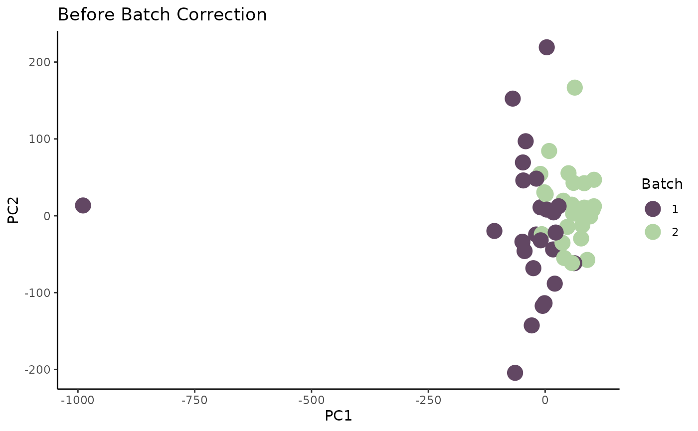

There is a very obvious outlier in our data. We can quantitatively identify this outlier by identifying samples that lie beyond a threshold of 1.5 * IQR of the first and fourth quartiles.

# extract PC scores for given PC
scores <- org_pca[["PC1"]]

# compute IQR of given PC
iqr <- IQR(scores)

# compute upper and lower thresholds
upp_thres <- quantile(scores, 0.75) + 1.5 * iqr
low_thres <- quantile(scores, 0.25) - 1.5 * iqr

# print samples with values beyond threshold
outlier <- rownames(org_pca)[which(scores < low_thres | scores > upp_thres)]
paste("Outlier for PC1:", outlier) |> print()

## [1] "Outlier for PC1: T-47D"

Let’s remove T-47D and re-plot our data.

# remove outlier
outlier <- "T-47D"
tpm_matrix[[outlier]] <- NULL

# redo PCA and plotting
org_pca <- prcomp(t(tpm_matrix))$x |> as.data.frame()
org_pca$Batch <- meta$batchid[match(rownames(org_pca), meta$sampleid)] |> as.factor()

p1 <- ggplot(org_pca) +
  geom_point(aes(x = PC1, y = PC2, color = Batch), size = 5) +
  scale_color_manual(values = c("#624763", "#B1D3A3")) +
  theme_classic() +
  ggtitle("Before Batch Correction")

p1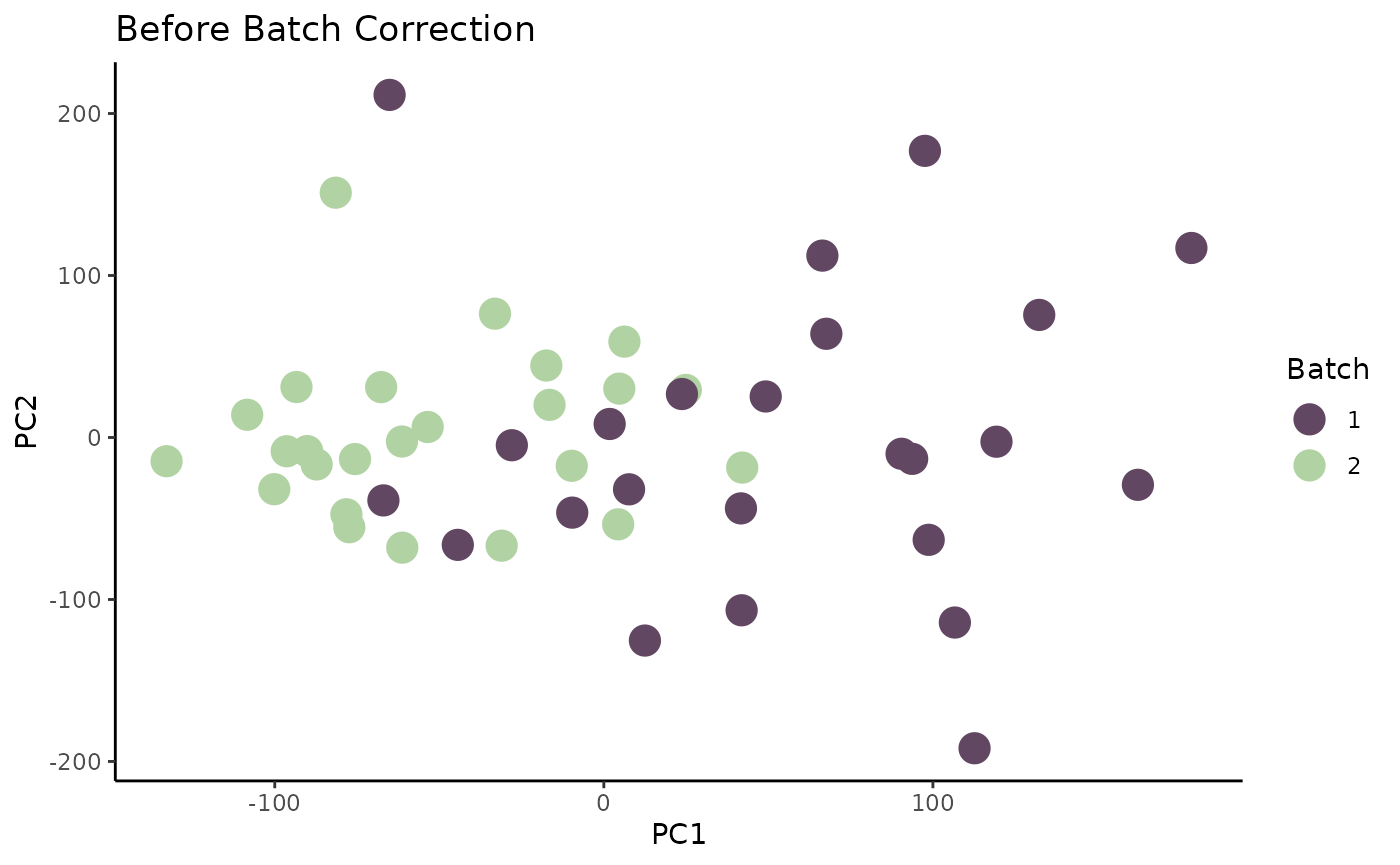

Now that the outlier is removed, we have a better visualization of the data. It is very evident that the data points (samples) tend to cluster by batch. This is indicative of a potential batch effect.

Adjusting for known batches

When we have a known batch, we can adjust for it directly. One method is to use the ComBat() function from the sva package.

# adjust for known batch
adj_tpm_matrix <- ComBat(
  dat = tpm_matrix,
  batch = as.factor(meta$batchid[match(colnames(tpm_matrix), meta$sampleid)]),
  par.prior = TRUE,
  prior.plots = FALSE
)

## Found2batches

## Adjusting for0covariate(s) or covariate level(s)

## Standardizing Data across genes

## Fitting L/S model and finding priors

## Finding parametric adjustments

## Adjusting the Data

adj_tpm_matrix[1:5, 1:5]

##           NCI-H23   HOP-62    SNB-75 HL-60(TB)     A-549
## GENE001 81.991219 68.65465 94.477925  46.14868  9.844954
## GENE003 78.009018 94.55152  9.221893  94.18421 46.353576
## GENE004  2.112512 81.72158 19.570898  48.84136 82.434411
## GENE005 53.126927 73.84929 84.808130  57.36965 71.508314
## GENE006 25.252026 67.80845 80.339726 106.46140 48.702080

We can now perform PCA and visualize on our adjusted TPM counts matrix. We will compare the results to the original PCA visualization.

Don’t forget to transpose the adjusted counts matrix!

# perform PCA on adjusted matrix

adj_pca <- prcomp(t(adj_tpm_matrix))$x |> as.data.frame()
adj_pca$Batch <- meta$batchid[match(rownames(adj_pca), meta$sampleid)] |> as.factor()

# create scatter plot
p2 <- ggplot(adj_pca) +
  geom_point(aes(x = PC1, y = PC2, color = Batch), size = 5) +
  scale_color_manual(values = c("#624763", "#B1D3A3")) +
  theme_classic() +
  ggtitle("After Batch Correction")

# plot both plots side by side for comparison
ggarrange(p1, p2, ncol = 2)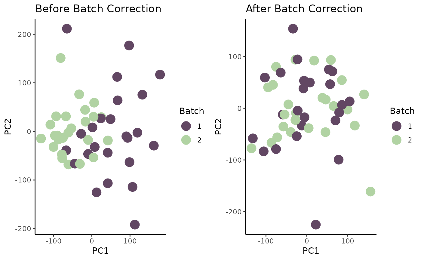

For downstream pharmacogenomic analysis (or any other bioinformatic analysis), the batch-corrected expression matrix should be used.

Jermiah J. Joseph

Julia Nguyen

Lab 2 Overview

Instructor(s) name(s) and contact information

Learning goals

Learning objectives

Setup

Use Cases for PharmacoGx

Understanding the PharmacoSet Data Structure

Metadata

View the sample slot

View the treatment slot

Molecular Profiles

MultiAssayExperiment and SummarizedExperiment

View the molecularProfiles slot

Treatment Response

View the treatmentResponse slot

Subsetting a PharmacoSet

Subset by sampleNames and/or treatmentNames

Subsetting using sample and treatment metadata

Computing over a TreatmentResponseExperiment

Aggregating over the TreatmentResponseExperiment

Plotting the number of replicates

Summarize over technical replicates

Endoaggregate

Computing profiles

Quality Control of Pharmacogenomic Datasets

Checking for missing values

Principal component analysis for outlier removal

Adjusting for known batches

Understanding the `PharmacoSet` Data Structure

View the `sample` slot

View the `treatment` slot

`MultiAssayExperiment` and `SummarizedExperiment`

View the `molecularProfiles` slot

View the `treatmentResponse` slot

Subsetting a `PharmacoSet`

Subset by `sampleNames` and/or `treatmentNames`

Subsetting using `sample` and `treatment` metadata

Computing over a `TreatmentResponseExperiment`

Aggregating over the `TreatmentResponseExperiment`

`Endoaggregate`