Module 3: Pharmacogenomics for biomarker discovery – Basic analysis

Jermiah J. Joseph

Princess Margaret Cancer Centre
jermiah.joseph@uhn.ca

Nikta Feizi

Princess Margaret Cancer Centre
nikta.feizi@uhn.ca

Julia Nguyen

Princess Margaret Cancer Centre
julia.nguyen@uhn.ca

18 October 2024

Source: vignettes/Module3.Rmd

Module3.Rmd

Overview

Lab 3 Overview

Instructor(s) name(s) and contact information

Jermiah J. Joseph jermiah.joseph@uhn.ca
Nikta Feizi <>
Julia Nguyen julia.nguyen@uhn.ca

PharmacoGx Package Overview

PharmacoGx: An R package for analyzing pharmacogenomic datasets.

Key Functions:

Install and Load PharmacoGx

install.packages("BiocManager")
BiocManager::install("PharmacoGx")
library(PharmacoGx)

Download a PharmacoSet

availablePSets()
GDSC <- downloadPSet("GDSC_2020(v2-8.2)")
# downloadPSet(): Download pharmacogenomic datasets.

Extract Drug Response Data

drug_response <- summarizeSensitivityProfiles(GDSC, sensitivity.measure='aac_recomputed')
# summarizeSensitivityProfiles(): Summarize drug response data.

Extract Gene Expression Data

gene_expr <- summarizeMolecularProfiles(GDSC, mDataType='rna') 
gene_expr_mtx <- assay(gene_expr)

Data Retrieval:

availablePSets(): Lists available pharmacogenomic datasets.

Downloading Multiple PharmacoSets:

PSet.list <- lapply(c("GDSC", "CCLE", "CTRP"), downloadPSet)
names(PSet.list) <- c("GDSC", "CCLE", "CTRP")

Accessing Molecular Profiles:

molecular.data <- lapply(PSet.list, function(pset) {
  summarizeMolecularProfiles(pset, mDataType = 'rna')
})

Introduction

In this workshop, we will explore data integration and comparative analysis using the PharmacoGx package, focusing on the GDSC and CCLE datasets. Specifically, we will cover drug sensitivity comparisons using AUC and IC50 measures and investigate correlations between gene expression profiles. This R Markdown file is designed to give participants hands-on experience with data exploration and interpretation.

Learning Objectives

Learn how to load and handle data from the GDSC and CCLE datasets.
Understand how to summarize drug sensitivity profiles and molecular data.
Perform correlations to assess concordance between cell line datasets.
Visualize and interpret the results of statistical tests.

Exploring GDSC and CCLE Datasets

Load GDSC and CCLE Datasets

We will use the GDSCsmall and CCLEsmall sample datasets provided by PharmacoGx to compare the two data sources.

data("GDSCsmall")
data("CCLEsmall")
GDSCsmall

## <PharmacoSet>
## Name: GDSC 
## Date Created: Mon Aug 24 15:18:23 2015 
## Number of samples:  10 
## Molecular profiles: 
## RNA :
##   Dim: 300, 11 
## rna2 :
##   Dim: 300, 9 
## mutation :
##   Dim: 70, 10 
## Treatment response: Drug pertubation:
##    Please look at pertNumber(cSet) to determine number of experiments  for each drug-sample combination.
## Drug sensitivity:
##    Number of Experiments:  972 
##    Please look at sensNumber(cSet) to determine number of  experiments for each drug-sample combination.

Find Common Genes Between GDSC and CCLE

The first step in comparing datasets is to find shared features between them. Here, we identify the genes that are present in both datasets.

commonGenes <- intersect(fNames(GDSCsmall, "rna"), fNames(CCLEsmall, "rna"))
length(commonGenes)

## [1] 41

There are 41 genes that are common between the RNA profiles of the GDSC and CCLE datasets.

Identify Common Cell Lines and Drugs

Next, we identify the common cell lines and drugs between GDSC and CCLE.

common <- intersectPSet(
  list("CCLE" = CCLEsmall, "GDSC" = GDSCsmall),
  intersectOn = c("cell.lines", "drugs"),
  strictIntersect = TRUE
)

## Intersecting large PSets may take a long time ...

cellNames(common[[1]])

## [1] "22RV1"    "23132-87" "5637"     "639-V"    "647-V"    "697"      "769-P"   
## [8] "786-0"    "8-MG-BA"

length(cellNames(common[[1]]))

## [1] 9

There are 9 common samples between GDSC and CCLE. The intersectPSet function returns a list of the two PSets subsetted to include only the common cell lines.

common

## $CCLE
## <PharmacoSet>
## Name: CCLE 
## Date Created: Fri Nov  6 14:00:53 2015 
## Number of samples:  9 
## Molecular profiles: 
## RNA :
##   Dim: 50, 9 
## RNAseq :
##   Dim: 50, 9 
## mutation :
##   Dim: 1667, 9 
## CNV :
##   Dim: 50, 7 
## Treatment response: Drug pertubation:
##    Please look at pertNumber(cSet) to determine number of experiments  for each drug-sample combination.
## Drug sensitivity:
##    Number of Experiments:  102 
##    Please look at sensNumber(cSet) to determine number of  experiments for each drug-sample combination.
## 
## $GDSC
## <PharmacoSet>
## Name: GDSC 
## Date Created: Mon Aug 24 15:18:23 2015 
## Number of samples:  9 
## Molecular profiles: 
## RNA :
##   Dim: 300, 10 
## rna2 :
##   Dim: 300, 9 
## mutation :
##   Dim: 70, 9 
## Treatment response: Drug pertubation:
##    Please look at pertNumber(cSet) to determine number of experiments  for each drug-sample combination.
## Drug sensitivity:
##    Number of Experiments:  79 
##    Please look at sensNumber(cSet) to determine number of  experiments for each drug-sample combination.

Notice that most of the molecular profiles are subsetted to include the 9 common samples. Some odd cases include RNA from GDSC which has a technical replicate (hence 10 samples) and CNV from CCLE which is missing CNV profiles for two of the nine cell lines.

Summarize Drug Sensitivity Profiles

We summarize drug sensitivity profiles (AUC and IC50) for each dataset. The summary.stat parameter can be set to different statistical metrics such as mean, median, etc. Here, we use the median for summarizing the sensitivity.

# Summary statistics for AUC
GDSC.auc <- summarizeSensitivityProfiles(
  common$GDSC,
  sensitivity.measure = "auc_published",
  summary.stat = "median",
  verbose = FALSE
)
CCLE.auc <- summarizeSensitivityProfiles(
  common$CCLE,
  sensitivity.measure = "auc_published",
  summary.stat = "median",
  verbose = FALSE
)

# Summary statistics for IC50
GDSC.ic50 <- summarizeSensitivityProfiles(
  common$GDSC,
  sensitivity.measure = "ic50_published",
  summary.stat = "median",
  verbose = FALSE
)
CCLE.ic50 <- summarizeSensitivityProfiles(
  common$CCLE,
  sensitivity.measure = "ic50_published",
  summary.stat = "median",
  verbose = FALSE
)
CCLE.auc |> head()

##               22RV1 23132-87      5637     639-V 647-V       697      769-P
## PD-0325901 0.385000       NA 0.1708125 0.3088750    NA 0.2291000 0.23250000
## 17-AAG     0.372460       NA 0.4828250 0.4877500    NA 0.3420875 0.40937500
## Nilotinib  0.000000       NA 0.0072625 0.0710125    NA 0.1573375 0.00000000
## PHA-665752 0.094375       NA 0.0000000 0.0194000    NA 0.1609750 0.09427143
## lapatinib  0.036125       NA 0.2212250 0.0066000    NA 0.0453250 0.16475000
## Nutlin-3   0.076925       NA 0.0000000 0.0666625    NA 0.2588125 0.08598571
##                 786-0   8-MG-BA
## PD-0325901 0.13862500 0.0758750
## 17-AAG     0.44162500 0.4426500
## Nilotinib  0.07501250        NA
## PHA-665752 0.07408625 0.3962500
## lapatinib  0.12987500 0.0547625
## Nutlin-3   0.00000000 0.0655125

We can visualize the distribution of drug sensitivity profiles to compare between the two psets.

First we quickly reformat the data into a long format to facilitate plotting. We use the melt() function from the reshape2 package.

CCLE_toPlot <- melt(CCLE.auc)
colnames(CCLE_toPlot) <- c("Drug", "Gene", "AUC")

CCLE_toPlot |> head()

##         Drug  Gene      AUC
## 1 PD-0325901 22RV1 0.385000
## 2     17-AAG 22RV1 0.372460
## 3  Nilotinib 22RV1 0.000000
## 4 PHA-665752 22RV1 0.094375
## 5  lapatinib 22RV1 0.036125
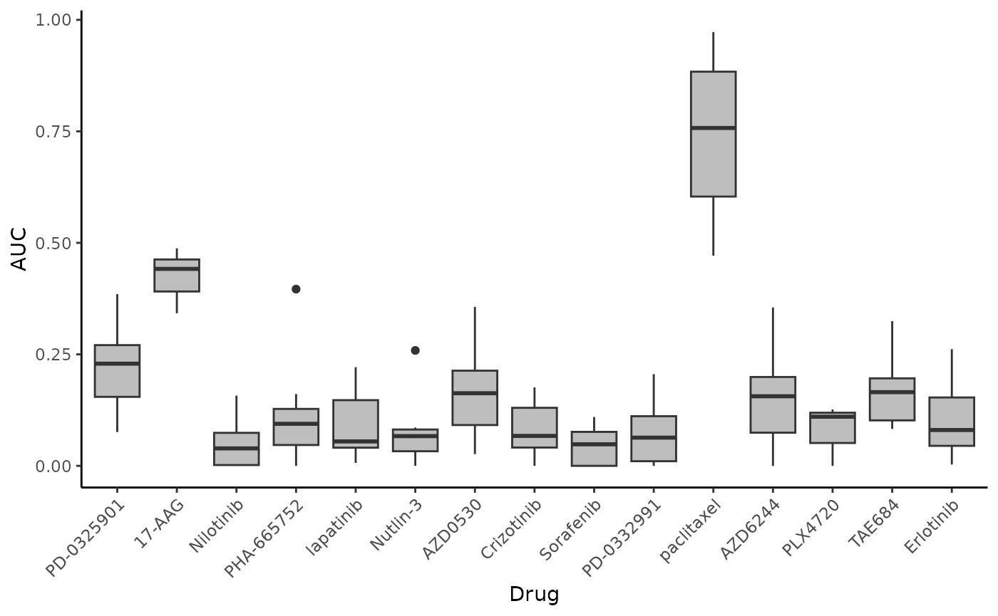
## 6   Nutlin-3 22RV1 0.076925

Next, we can create a quick box plot to visualize the AUC distributions per drug.

ggplot(CCLE_toPlot, aes(x = Drug, y = AUC)) + geom_boxplot(fill = "grey") +
  theme_classic() + theme(axis.text.x = element_text(angle = 45, hjust = 1)) #rotate x-axis labels

## Warning: Removed 33 rows containing non-finite outside the scale range
## (`stat_boxplot()`).

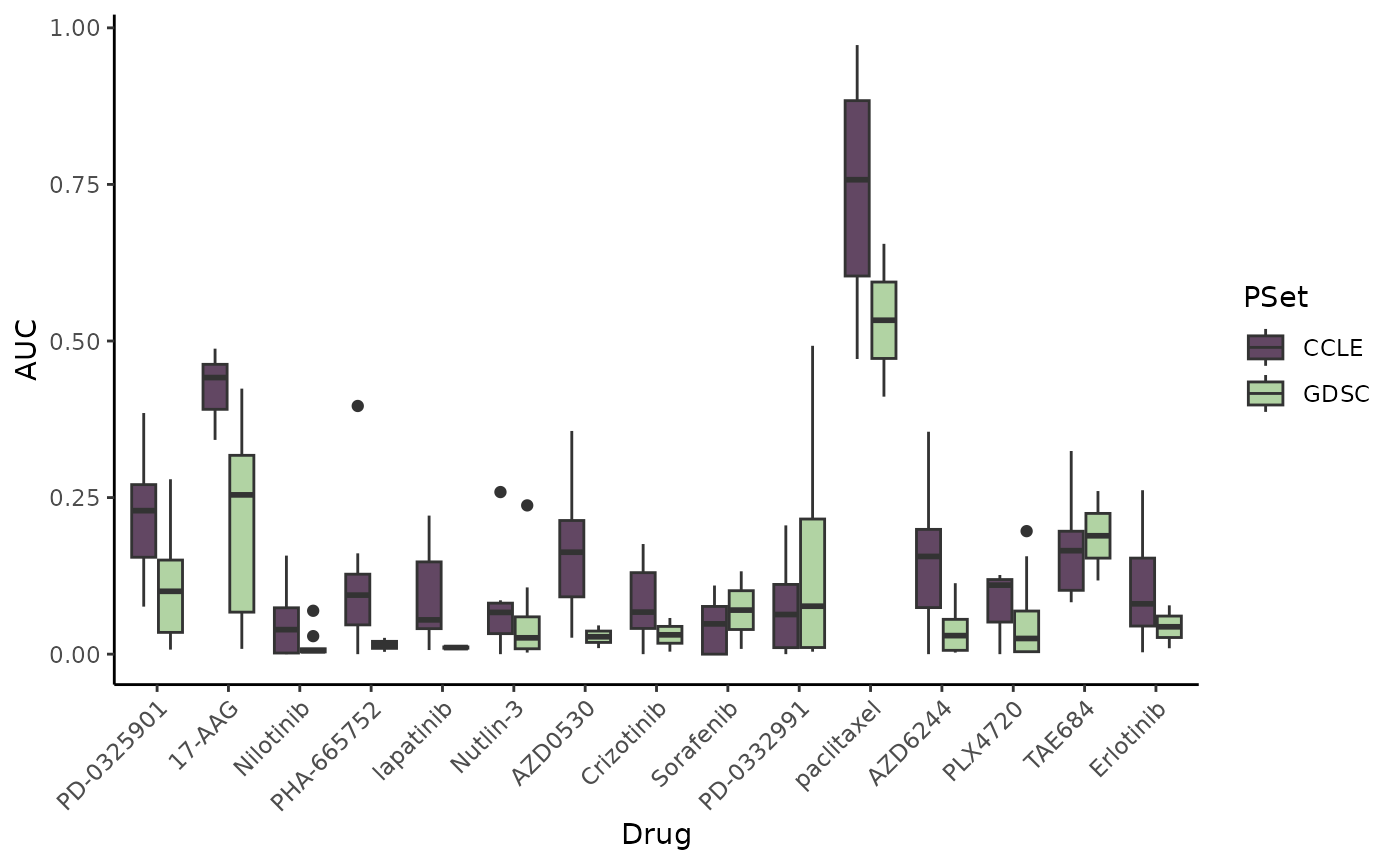
Let’s do this again but with the GDSC PSet so we can compare the two

# format the CCLE sensitivity data
GDSC_toPlot <- melt(GDSC.auc)
colnames(GDSC_toPlot) <- c("Drug", "Gene", "AUC")

# merge the two pset dataframes
GDSC_toPlot$PSet <- "GDSC"
CCLE_toPlot$PSet <- "CCLE"
merge_toPlot <- rbind(GDSC_toPlot, CCLE_toPlot)

# plot to compare AUC distribution between PSets
ggplot(merge_toPlot, aes(x = Drug, y = AUC)) + geom_boxplot(aes(fill = PSet)) +
  scale_fill_manual(values = c("#624763", "#B1D3A3")) + theme_classic() + 
  theme(axis.text.x = element_text(angle = 45, hjust = 1)) #rotate x-axis labels

## Warning: Removed 89 rows containing non-finite outside the scale range
## (`stat_boxplot()`).

Preclinical drug response data is fairly noisy, hence the variation we see between the two datasets. However, we do see some commonalities in distribution.

Summarize Gene Expression Profiles

We summarize gene expression data for the genes that are common between GDSC and CCLE.

GDSCexpression <- summarizeMolecularProfiles(
  common$GDSC, cellNames(common$GDSC),
  mDataType = "rna", features = commonGenes, verbose = FALSE
) |> assay()
CCLEexpression <- summarizeMolecularProfiles(
  common$CCLE, cellNames(common$CCLE),
  mDataType = "rna", features = commonGenes, verbose = FALSE
) |> assay() 

GDSCexpression |> head()

##                     22RV1  23132-87      5637     639-V     647-V       697
## ENSG00000000003  5.890740  6.243345 10.018953  9.653157 10.039302  5.215355
## ENSG00000000005  4.448758  4.335738  4.108065  4.014940  4.250878  4.367339
## ENSG00000000419 10.427302 11.045576 11.611295 11.604278 11.248686 10.572231
## ENSG00000000457  5.905884  6.900556  5.684007  5.392485  5.748209  5.934834
## ENSG00000000460  6.010605  5.433439  5.729120  5.439058  6.453635  6.342021
## ENSG00000000938  4.410785  4.329849  4.397001  4.176387  4.275824  4.618786
##                    769-P     786-0   8-MG-BA
## ENSG00000000003 8.615450  7.304893  7.994002
## ENSG00000000005 4.722970  4.235424  4.447925
## ENSG00000000419 9.927782 10.825907 10.759706
## ENSG00000000457 6.475836  5.087249  4.994176
## ENSG00000000460 5.999142  5.001772  6.073944
## ENSG00000000938 5.003250  4.443563  4.797094

Here, you could do PCA on the profiles to quickly check the data. We will skip this step in the interest of time.

Correlation Analysis Between GDSC and CCLE

We perform correlation analysis to examine the relationship between gene expression, AUC, and IC50 measures across the GDSC and CCLE datasets using Spearman’s correlation.

# get common cell line names
cc <- cellNames(common[[1]])

# correlation of gene expression across common cell lines
ge.cor <- sapply(cc, function(x, d1, d2) {
  stats::cor(
    d1[, x], d2[, x],
    method = "spearman", use = "pairwise.complete.obs"
  )
}, d1 = GDSCexpression, d2 = CCLEexpression)

ge.cor

##     22RV1  23132-87      5637     639-V     647-V       697     769-P     786-0 
## 0.8658537 0.8844948 0.8935540 0.9202091 0.9106272 0.8893728 0.8939024 0.8681185 
##   8-MG-BA 
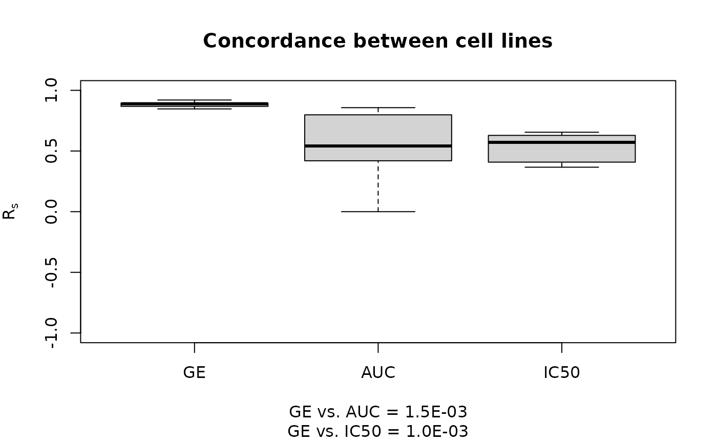
## 0.8470383

We can see that the RNA-Seq expression values are highly correlated across the common cell lines.

Let’s take a look at the correlation of drug response, starting with IC50 values.

# quick look at the CCLE IC50 data
CCLE.ic50 |> head()

##                22RV1 23132-87       5637     639-V 647-V       697     769-P
## PD-0325901 8.0000000       NA 8.00000000 8.0000000    NA 8.0000000 1.4542717
## 17-AAG     0.3297017       NA 0.07082279 0.1500945    NA 0.4225712 0.1517988
## Nilotinib  8.0000000       NA 7.47535467 8.0000000    NA 1.9104344 8.0000000
## PHA-665752 8.0000000       NA 8.00000000 8.0000000    NA 3.2754419 7.1504111
## lapatinib  7.8473053       NA 2.30776763 8.0000000    NA 0.8494762 1.0574611
## Nutlin-3   8.0000000       NA 8.00000000 8.0000000    NA 1.8905237 5.5913019
##                786-0   8-MG-BA
## PD-0325901 8.0000000 8.0000000
## 17-AAG     0.2795302 0.2349526
## Nilotinib  8.0000000        NA
## PHA-665752 8.0000000 8.0000000
## lapatinib  7.1780353 5.2266199
## Nutlin-3   8.0000000 8.0000000

# correlation of IC50 values across common drugs and cell lines
ic50.cor <- sapply(cc, function(x, d1, d2) {
  stats::cor(
    d1[, x], d2[, x],
    method = "spearman", use = "pairwise.complete.obs"
  )
}, d1 = GDSC.ic50, d2 = CCLE.ic50)

ic50.cor

##     22RV1  23132-87      5637     639-V     647-V       697     769-P     786-0 
## 0.4082483        NA 0.5713800 0.4082483        NA 0.6273461 0.6300619 0.6546537 
##   8-MG-BA 
## 0.3664850

Notice that we have some NA values in the original CCLE IC50 dataset and in the correlation results.

The pairwise.complete.obs argument used in the cor() function ensures that only complete observations (i.e. numeric values that are not NA) are included in the pairwise correlations.

Since 23132-87 and 647-V are all NA values, no spearman correlation was computed.

We can quickly compute the correlation for AUC as well.

# correlation of AUC values across common drugs and cell lines
auc.cor <- sapply(cc, function(x, d1, d2) {
  stats::cor(
    d1[, x], d2[, x],
    method = "spearman", use = "pairwise.complete.obs"
  )
}, d1 = GDSC.auc, d2 = CCLE.auc)

auc.cor

##     22RV1  23132-87      5637     639-V     647-V       697     769-P     786-0 
## 0.0000000        NA 0.7748062 0.8214286        NA 0.3750000 0.8571429 0.4638168 
##   8-MG-BA 
## 0.5414447

Statistical Comparison

We compare the correlations using Wilcoxon signed-rank tests to see if there are significant differences between the gene expression correlations and the drug sensitivity correlations.

w1 <- stats::wilcox.test(
  x = ge.cor, y = auc.cor, conf.int = TRUE, exact = FALSE
)
w2 <- stats::wilcox.test(
  x = ge.cor, y = ic50.cor, conf.int = TRUE, exact = FALSE
)

w1

## 
##  Wilcoxon rank sum test with continuity correction
## 
## data:  ge.cor and auc.cor
## W = 62, p-value = 0.001496
## alternative hypothesis: true location shift is not equal to 0
## 95 percent confidence interval:
##  0.06309566 0.51857816
## sample estimates:
## difference in location 
##               0.347967

w2

## 
##  Wilcoxon rank sum test with continuity correction
## 
## data:  ge.cor and ic50.cor
## W = 63, p-value = 0.001024
## alternative hypothesis: true location shift is not equal to 0
## 95 percent confidence interval:
##  0.2407670 0.4857055
## sample estimates:
## difference in location 
##              0.3179657

# Display p-values
ss <- sprintf("GE vs. AUC = %.1E\nGE vs. IC50 = %.1E", w1$p.value, w2$p.value)
cat(ss)

## GE vs. AUC = 1.5E-03
## GE vs. IC50 = 1.0E-03

Boxplot Visualization

The results are visualized using boxplots to compare the correlations across gene expression, AUC, and IC50.

boxplot(list("GE" = ge.cor, "AUC" = auc.cor, "IC50" = ic50.cor),
  main = "Concordance between cell lines",
  ylab = expression(R[s]),
  sub = ss,
  ylim = c(-1, 1),
  col = "lightgrey",
  pch = 20,
  border = "black"
)

Statistical Analysis for Drug Response Associations

In this final section, we will be focusing on computing the association between a feature of interest and drug response in order to identify predictive biomarkers.

Let’s begin by selecting a feature and drug of interest to explore.

commonGenes |> head()

## [1] "ENSG00000000003" "ENSG00000000005" "ENSG00000000419" "ENSG00000000457"
## [5] "ENSG00000000460" "ENSG00000000938"

feature <- "ENSG00000000003"

common$GDSC@treatment |> rownames()

##  [1] "PD-0325901" "17-AAG"     "Nilotinib"  "PHA-665752" "lapatinib" 
##  [6] "Nutlin-3"   "AZD0530"    "Crizotinib" "Sorafenib"  "PD-0332991"
## [11] "paclitaxel" "AZD6244"    "PLX4720"    "TAE684"     "Erlotinib"

drug <- "PD-0325901"

Next, we need to extract the vector of gene expression for our chosen feature and drug response for our chosen drug. Let’s do this for the GDSC dataset.

Gene <- GDSCexpression[feature,]
Drug <- GDSC.auc[drug,]

Gene

##     22RV1  23132-87      5637     639-V     647-V       697     769-P     786-0 
##  5.890740  6.243345 10.018953  9.653157 10.039302  5.215355  8.615450  7.304893 
##   8-MG-BA 
##  7.994002

Drug

##    22RV1 23132-87     5637    639-V    647-V      697    769-P    786-0 
## 0.029649 0.122911 0.007242 0.279261 0.100351 0.049681 0.179831 0.150231 
##  8-MG-BA 
## 0.034754

Notice that the PSet has already kept the samples ordered across the various profiles.

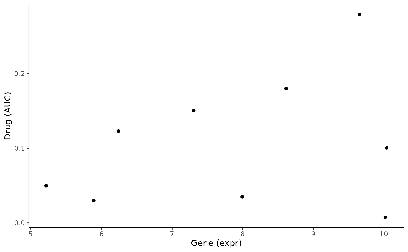
Before we compute the associations, we can quickly plot the two variables to visualize their relationship.

# create datafarme to plot
toPlot <- data.frame(Gene = Gene, Drug = Drug)

ggplot(toPlot, aes(x = Gene, y = Drug)) + geom_point() +
  theme_classic() + labs(x = "Gene (expr)", y = "Drug (AUC)")

From the scatter plot, we see a weak positive correlation. Let’s see if this is reflected in our association analyses.

Concordance Index

Fist, we will compute the association between the gene expression data and drug response. We will use the concordance.index function from the survcomp package.

ci <- survcomp::concordance.index(
  as.numeric(Drug),                   # drug vector
  surv.time = as.numeric(Gene),       # gene vector
  surv.event = rep(1,length(Gene)),   
  outx = TRUE, method="noether", na.rm = TRUE
)

cat("Concordance Index:", ci$c.index, "\n",
    "P-value:", ci$p.value, "\n",
    "Standard Error:", ci$se, "\n", 
    "Upper CI:", ci$upper,"\n",
    "Lower CI:", ci$lower)

## Concordance Index: 0.4166667 
##  P-value: 0.07592696 
##  Standard Error: 0.04695301 
##  Upper CI: 0.5086929 
##  Lower CI: 0.3246404

The concordance index tells us there is a weak inverse association between the gene expression and the drug response.

Pearson’s Correlation Coefficient

Using the same feature and drug, let’s compute the association again but this time using Pearson’s correlation.

ps <- cor.test(
  x = Gene,
  y = Drug,
  alternative = "two.sided",
  method = "pearson"
)

cat("Pearson's correlation:", ps$estimate, "\n",
    "P-value:", ci$p.value, "\n",
    "Confidence Interval:", ps$conf.int)

## Pearson's correlation: 0.2937677 
##  P-value: 0.07592696 
##  Confidence Interval: -0.4601228 0.8015157

The Pearson’s correlation tells us there is a (very) weak positive linear relationship between the gene expression and the drug response.

Notice the slight difference in interpretation between the concordance index and the Pearson’s correlation.

Drug Sensitivity Signatures (PharmacoGx)

The last method we will explore is a built-in function from the PharmacoGx package called drugSensitivitySig. This function takes a PharmacoSet along with a list of drugs and features, then computes the association between the feature expression and drug response for each pair.

Let’s first select the first 3 genes and drugs as our features & drugs of interest:

features <- commonGenes[1:3]
drugs <- rownames(common$GDSC@treatment)[1:3]

features

## [1] "ENSG00000000003" "ENSG00000000005" "ENSG00000000419"

drugs

## [1] "PD-0325901" "17-AAG"     "Nilotinib"

Now we can calculate the drug sensitivity signature using the vector of genes and drugs for the GDSC dataset. Note that this gene-drug signature is based on univariable analysis.

# gene expression signature
sig.rna <- drugSensitivitySig(
  object = GDSCsmall,
  mDataType = "rna",
  drugs = drugs,
  features = features,
  sensitivity.measure = "auc_published",
  molecular.summary.stat = "median",
  sensitivity.summary.stat = "median",
  modeling.method = "pearson",
  verbose = FALSE
)
sig.rna@.Data[,,c(1,5)]

## , , estimate
## 
##                  PD-0325901     17-AAG  Nilotinib
## ENSG00000000003 -0.18840373 -0.2369481  0.8554590
## ENSG00000000005 -0.14409315 -0.4756331  0.7875267
## ENSG00000000419 -0.02890968  0.5466780 -0.8239237
## 
## , , pvalue
## 
##                 PD-0325901    17-AAG Nilotinib
## ENSG00000000003  0.8793373 0.8477058 0.3465502
## ENSG00000000005  0.9079470 0.6844380 0.4227225
## ENSG00000000419  0.9815930 0.6317843 0.3835609

The output is a 3D array of genes x drugs x metric. Outputted are the estimate and pvalue. Feel free to explore the other array components in sig.rna@.Data.

This function is a powerful method for investigating the univariate relationship between multiple molecular features and drugs.

Let’s do the same for mutations, we’ll do a quick example using one gene and drug from the CCLE dataset.

# mutation signature
sig.mut <- drugSensitivitySig(
  object = CCLEsmall,
  mDataType = "mutation",
  drugs = "PD-0325901",
  features = "BRAF",
  sensitivity.measure = "auc_published",
  molecular.summary.stat = "and",
  sensitivity.summary.stat = "median",
  verbose = FALSE
)
sig.mut@.Data[,,c(1,6)]

##     estimate       pvalue 
## 8.251857e-01 1.612881e-09

Univariate vs Multivariate Analysis

For the final section of this lab, we will explore univariate vs multivariate linear modeling. Let’s start with a simple univariate linear model using the same Gene and Drug vector from earlier.

Univariate Analysis

Recall Gene is the RNA expression vector of ENSG00000000005 and Drug is the drug response vector (AUC) for PD-0325901 in the GDSC dataset.

lm(Drug ~ Gene) |> summary()

## 
## Call:
## lm(formula = Drug ~ Gene)
## 
## Residuals:
##      Min       1Q   Median       3Q      Max 
## -0.12867 -0.04835 -0.01884  0.05239  0.14848 
## 
## Coefficients:
##              Estimate Std. Error t value Pr(>|t|)
## (Intercept) -0.004639   0.139300  -0.033    0.974
## Gene         0.014028   0.017253   0.813    0.443
## 
## Residual standard error: 0.08965 on 7 degrees of freedom
## Multiple R-squared:  0.0863, Adjusted R-squared:  -0.04423 
## F-statistic: 0.6612 on 1 and 7 DF,  p-value: 0.4429

Let’s break down this output:

Residuals: the difference between the predicted y (drug response) values and the actual y values. A larger range suggests the model may not be a good fit of the data.

Coefficients: the parameters of the model. - Estimate can be considered the effect size. Specifically, it is the one-unit change in the y variable (drug response) per one-unit change in the x variable (gene expression). The estimate from our drug~gene association is 0.014028. - Pr(>|t|) is the corresponding p-value for each estimate. The p-value from our drug~gene association test is 0.443.

Note: If any of the coefficients had met the p-value < 0.05 significance threshold, you would have seen * beside the estimate (unfortunately, this association does not meet this threshold).

Let’s see if we can make a multi-variate model with better performance.

# get another gene vector
commonGenes[2]

## [1] "ENSG00000000005"

Gene2 <- GDSCexpression[commonGenes[2],]

# multi-variate model
lm(Drug ~ Gene + Gene2) |> summary()

## 
## Call:
## lm(formula = Drug ~ Gene + Gene2)
## 
## Residuals:
##      Min       1Q   Median       3Q      Max 
## -0.13292 -0.04715 -0.02147  0.04840  0.14047 
## 
## Coefficients:
##             Estimate Std. Error t value Pr(>|t|)
## (Intercept)  0.15618    0.84445   0.185    0.859
## Gene         0.01251    0.02017   0.620    0.558
## Gene2       -0.03441    0.17780  -0.194    0.853
## 
## Residual standard error: 0.09653 on 6 degrees of freedom
## Multiple R-squared:  0.09197,    Adjusted R-squared:  -0.2107 
## F-statistic: 0.3038 on 2 and 6 DF,  p-value: 0.7487

The second gene feature we are adding to our model is ENSG00000000005.

Take a look at the output, comparing it to the previous model we ran. Do you think that adding an additional gene has improved model performance?

Individual Practice

For the remainder of the lab, please explore the associations between other features and drug response. Try using the CCLE pset too!